Well, this would not be a popular science blog about the exact sciences if I did not try, at least once, to speak with some authority about a neighboring field that sits outside the scope of my own domain. The idea of this post is to talk about statistics and psychology. Despite the sources, it is still terrain I do not master, so I will lean on them as much as possible to avoid making any unfounded claims.
The Sally Clark case and the prosecutor's fallacy
To ground the discussion, let's start with the classic Sally Clark case and the infamous prosecutor's fallacy, in which two statistical errors were committed, broadly, throughout a trial, by practically everyone present, from the jury to the judge.
It was assumed that the chance of a newborn suffering sudden death (given the mother's profile: over 26 years old, non-smoker) was around 1 in 8,000 and that, consequently, the chance of this happening to both of Sally Clark's babies would be 1 in 73 million. Here we already have the first error, a classic in statistics: assuming independence of the data.
The chance of a newborn being affected by this may well be 1 in 8,000, but that statistic serves to ground the field's understanding of a given subject (statistics a priori). It does not serve to assess the chance of something having happened, given that the event already occurred (statistics a posteriori). When assessing an individual case, there may be other n factors (risk group, family history, among others) that would raise or lower that statistic in that specific case.
More seriously still, when analyzing two siblings, you cannot simply multiply the numbers, because independence here is not only not guaranteed but simply does not exist: several factors that would indicate sudden death in one of the children tend to repeat in the second. Thus, the "real" probability (considering the average statistic used to describe the population, but which does not necessarily describe particular cases) would be something between 1 in 150,000 and 1 in 350,000, roughly 100 times smaller than the initial statistic.
Even so, these values, on their own, say nothing. Statistics are just numbers that describe events. Using them is the job of specialists trying to understand phenomena. And this is where we reach the second problem: the prosecutor's fallacy.
On presenting the number (1 in 73 million) to the court, the jury understood, automatically, that the chance of Sally being innocent was precisely the chance of those rare events happening, since, otherwise, she would indeed have killed both. The statistic does not say that. It says far less than that. Even if we accept the number as true, the probability of both children dying, given that she is innocent (1 in 73 million), is not the probability that matters. What matters is the probability of Sally being innocent given that both children died, and, by the math, the difference is enormous.
The correct structure would be:
- H = Clark is guilty
- ¬H = Clark is innocent
- E = the observed evidence: both children died in infancy, in this pattern
On top of that, analyzing the number of a rare event without any reference could also, on its own, have led the jury astray. Rare as it is for this syndrome to occur twice, it is rarer still for a mother to murder both of her own babies, with that second probability being 4 to 9 times rarer. In the end, the homicide would be a less likely event than the death of two children in the same family from this kind of syndrome.
Probability and arithmetic are the same law, seen from afar
P(A∪B) = P(A) + P(B) − P(A∩B)P(A∩B) = P(A) × P(B|A)
These two lines are addition and multiplication, fully generalized. Ordinary arithmetic (a+b, a×b) is what remains when the correction terms vanish: when A∩B = ∅ (disjoint), or when P(B|A) = P(B) (independent).
The reason ordinary numbers get this "for free" is not that they satisfy independence or disjointness by some default assumption. It is that numbers were never events in a sample space to begin with. Overlap and conditioning are properties of sets of possibilities. An isolated number like 5 does not represent a slice of a sample space, so the question "does this overlap with something else?" does not even apply. There is no correction term to eliminate, because there was never a correction term present.
The correct picture, therefore, is not one of nesting (arithmetic as a subset that lives inside probability). It is one of degeneration: the laws of probability are the general case, and arithmetic is what results when you remove the one thing that made the correction terms necessary, that is, a shared sample space where events can overlap or influence one another. Remove that structure, and P(A)+P(B) simply becomes a+b, and P(A)×P(B) simply becomes a×b.
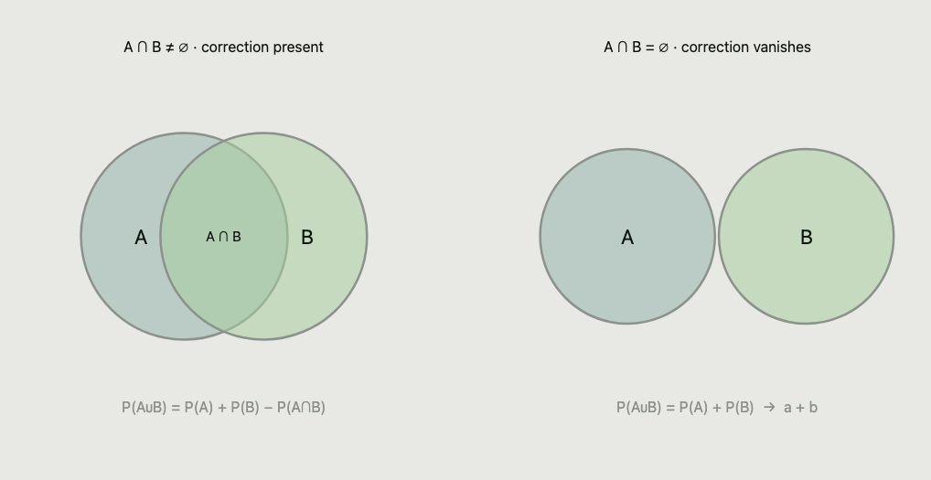
P(A∩B) is needed. When they are disjoint (right), that term vanishes and the sum of probabilities becomes the ordinary arithmetic sum, a + b.In the end, statistics seems to be a domain almost always misunderstood by everyone. Even though a jury is meant to broadly represent a population, and even though the medical expert consulted in the case had university training in basic statistics and knew how to read that kind of number, there were still widespread errors.
One point is worth highlighting: human knowledge has been accumulating for thousands of years, which eases our understanding of topics and widens our capacity for abstraction over them, since we have no way to understand every human domain. That is why we create abstractions and simplified models to teach people what we consider essential in each field. Because statistics is a relatively new field (much of the theory was developed in the last century, against millennia of other mathematical concepts), perhaps the abstractions we built (and are still building) have not fully captured the most intuitive way of thinking about these numbers.
The scientific part: the base rate fallacy
Moving into the more scientific part of this understanding, we have examples like Bar-Hillel's research on the base rate fallacy. It does not happen because people do not know math, or because they are incapable of integrating two sources of information. What actually happens is that people discard base rates because they feel those rates should be ignored as irrelevant to the judgment at hand. Two main factors make a piece of information "highly relevant":
- Specificity: information about a smaller, more specific subset dominates statistics about a general population.
- Causality: data suggesting a cause and effect relationship dominates data that looks like mere statistical coincidence.
The taxicab problem is the most famous example used to illustrate the fallacy. Participants were given the following scenario:
- In a city, 85% of the taxis belong to the Blue company and 15% to the Green company.
- A taxi is involved in a nighttime hit and run. A witness states that the taxi was Green.
- Tests show the witness has 80% accuracy identifying colors at night.
Most people answer something close to 80%, clinging to the witness's word and completely ignoring that green taxis are rare. Once you run the numbers with Bayes' theorem, though, the probability that the taxi really was green is only 41%.
Still within the same research, Bar-Hillel shows that people are able to use the base rate, as long as it seems as relevant as the case information. Similarly, there is the "intercom problem", a version analogous to the taxicab problem:
- Instead of a witness, the struck pedestrian heard the sound of a taxi intercom.
- It was reported that intercoms are installed in 80% of Green taxis and in 20% of Blue ones.
Here there is no causal witness, only two statistical distributions. On placing the taxis' base rate against the intercom indicator, the base rate fallacy vanished. Since neither piece of information seemed more causal or specific than the other, people started integrating the two. The median of the answers was 48%, remarkably close to the correct answer of 41%.
The a priori vs. a posteriori error
If an event has already happened, it, by definition, has a 100% probability of having occurred. For example: Sally Clark's two children died, that is a fact. The probability of the accomplished fact is 1, full stop. Faced with something that already occurred, we do not ask "how surprising was this event before I knew it happened?". The question that usually comes to mind is: "is this too rare to be coincidence?", and we answer looking backward, with the result already in hand. We are mixing up statistics a priori (the kind that describes the world before the die falls) with the a posteriori reading, made afterward, once we already know where it landed.
The hindsight bias, which Fischhoff documented in 1975, says that once we know how a story ends, we overestimate how predictable that ending was from the start. Using the opening case as a basis: after two children died, the jury silently reorganizes the whole past around that outcome, and what was a tragic and improbable chain of natural events starts to look like a plan. The known result contaminates the estimate of what was plausible before it existed.
That was exactly the trap the Sally Clark jury fell into. The 1 in 73 million number measured, at best, how surprising two deaths like those would be in a world where no one killed anyone. An event can be extremely rare and innocent at the same time. In fact, the murder of two babies by their mother is itself an extremely rare event, and, in some calculations, rarer still.
Where else this error hides
Gambler's fallacy. The roulette landed on red five times in a row, so "black is coming now". It is not. The roulette has no memory. Only your head does.
Hot hand. The basketball player hit four in a row: "he is on fire, pass it to him". Sometimes there is something real there. Sometimes it is just our habit of seeing pattern in a random sequence.
And perhaps the most everyday example of all is the Spotify shuffle. In the beginning, the app shuffled songs with a genuinely random algorithm: a uniform permutation, of the Fisher-Yates kind, in which any possible order had exactly the same chance of coming up. Statistically, it was the most correct "shuffle" one could ask for. The problem is that, in a truly random sequence, it is perfectly normal for two or three tracks by the same artist to land back to back, or for the same band to reappear a few minutes later. This is the expected behavior of chance, but, on hearing the same artist repeated, we conclude, with full conviction, that "the shuffle is broken" or that "it is not truly random".
Spotify's solution was to make the shuffle deliberately less random. Instead of drawing any order with equal probability, the algorithm started spreading each artist's songs across the playlist, preventing similar tracks from sitting close together, an approach inspired by color dispersion methods such as Martin Fiedler's. The result is a sequence that, from a mathematical point of view, is more organized and less random, but sounds far more "random" to whoever is listening.
We expect chance to distribute itself uniformly and regularly, and, when it forms clumps (as real chance always does), we read pattern, intent or defect where there is only luck. From the courtroom to the music app, the error is the same: confusing what randomness actually produces with what our intuition would like it to produce.
References
- Sally Clark, entry and timeline of the case. Wikipedia: en.wikipedia.org/wiki/Sally_Clark
- Royal Statistical Society, public statement on the Sally Clark case (2001): courthouselibrary.ca (PDF)
- The prosecutor's fallacy, with the Bayesian formalism: understandinguncertainty.org/node/545
- Bar-Hillel, M. (1980). "The base-rate fallacy in probability judgments." Acta Psychologica, 44(3): sciencedirect.com
- Gigerenzer, G. & Hoffrage, U. (1995). "How to improve Bayesian reasoning without instruction: Frequency formats." Psychological Review, 102(4), 684–704.
- Cosmides, L. & Tooby, J. (1996). "Are humans good intuitive statisticians after all? Rethinking some conclusions from the literature on judgment under uncertainty." Cognition, 58, 1–73.
- Barbey, A. K. & Sloman, S. A. (2007). "Base-rate respect: from ecological rationality to dual processes." Behavioral and Brain Sciences, 30(3).
- Fischhoff, B. (1975), the original study on hindsight bias, overview: en.wikipedia.org/wiki/Hindsight_bias
- Why the Spotify shuffle is not (and cannot be) truly random: howtogeek.com