Just One More Week and the Tale of Double or Nothing

The False Miracle

Everyone has seen it: the test for the feature that was going to change everything and bring in a billion in revenue. The test runs for two months. The team is anxious. When the results are presented, the big surprise arrives: the p-value came in at 0.06, just above the traditional 0.05 threshold.

The mood turns heavy. All those resources, all that time, all the hope invested in that brilliant idea seem lost. And then someone raises a hand and offers the solution, the light at the end of the tunnel, the rescue of the billion.

"What if we let the test run another week or two? Just to see if it finally crosses the line?"

Absolute silence, then the slow clap. Everyone pauses to admire the most brilliant idea that company has ever produced. Two weeks later, the "miracle" happens: the p-value drops to 0.048. The feature is approved and the hero is promoted. All that's left is to wait for the billions to roll in.

Everything looks perfect. But what may have actually happened is a false positive taking shape. How is that possible? To explain "counterintuitive" results in statistics, it always helps to reach for a classic: the Monty Hall Problem.

The Monty Hall Problem

You may not know it by name, but you have probably run into the concept somewhere, whether through that scene in the movie 21, or through a math-enthusiast friend trying to explain it (that last one may only happen to me and my friends).

The classic problem has the following elements: a TV host, a contestant, three doors, two of them hiding a goat and the winning one hiding a car. The contestant picks a door first; the host (who knows where the prize is) opens one of the two doors that were not picked and reveals a goat. Then he turns to the contestant and makes the offer: "Do you want to trade your door for the other one still closed?" Intuitively, nothing seems to have changed: a new choice, now at 50/50. That intuition is wrong, because it ignores the crucial fact that the host does not pick a door at random. Knowing where the prize is, he opens a door that does not contain it, and that adds information to the problem, which makes it a completely different problem.

Breaking the whole thing down:

1. Initial choice: you have a 1/3 chance of picking the car and a 2/3 chance of picking a goat.
2. The host: opens a goat door among the two you did not pick. If you picked a goat to begin with, he is forced to open the only other goat door, which inevitably leaves the car behind the remaining one.
3. Final decision: by switching, you invert the initial probabilities, ending up with a 2/3 chance of winning against only 1/3 if you stay.

If that still feels complicated, let's put Bayes' theorem, which governs this problem, on paper (or on the computer). That way we can see how adding a single piece of information completely changes the statistical problem.

Fix the scenario: you picked door 1 and the host opened door 3, revealing a goat. Call C₁, C₂ and C₃ the hypotheses that the car is behind each of the doors, all worth 1/3 before any reveal, and call E the evidence we just observed.

Bayes gives us:

• $P(E|C_1) = 1/2$, car behind the chosen door and goats behind doors 2 and 3.
• $P(E|C_2) = 1$, car behind door 2, so the host has to open door 3.
• $P(E|C_3) = 0$, he would never open the car's door.

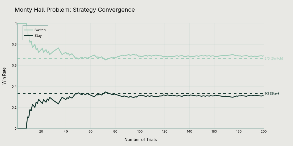
And the posteriors:

The original door keeps its original probability of 33.3%, and as a result the remaining door doubles to 66.7%. The host's action is not neutral; it transfers probability from the door he opens (which goes to zero) over to the other door.

If those calculations still feel otherworldly, we can turn to computational simulation to confirm the results, which consistently show that switching is the right call, since it gives roughly a 66.7% chance of winning while keeping the initial choice gives only 33.3%.

The Peeking Problem

When our protagonist opens the dashboard in week 8, sees a result close to the significance line and decides to let it run a bit longer, it looks harmless, much like switching or not switching in Monty Hall: someone holding information the others don't have makes an apparently neutral decision and, without announcing it, redistributes probability. The analogy has a limit. In Monty Hall, the host's information works in the contestant's favor, and opening an empty door lets us update the initial probability. In an A/B test the opposite happens: the stopping rule was fixed on paper, but the researcher himself broke it halfway through, and two extra weeks of data are, in fact, new information. What he lost was not information, it was the statistical guarantee that gave meaning to the p-value he computed. Monty Hall shows that new information changes a probability; peeking shows that whoever decides when to stop looking decides the result.

Every A/B test is born from four decisions made before any data comes in: the significance level α (type I error), the power 1−β, the minimum detectable effect (MDE), and the sample size, which is not a choice independent of the other three but the consequence of them combined with the smallest effect you care about detecting. That is a closed package, and it is valid under one condition only: you look at the result once. Peeking midway and deciding to continue based on what you saw turns one test into several, and at every look you hand chance another opportunity to cross the significance line out of pure luck. Chance takes every one of them.

Our hero took two looks. That puts his real α at around 8%, and the 4.8% p-value he found in week 10 sits below the wrong threshold. Once we use the true threshold of 8%, the test fails to establish a real effect, and the week 10 miracle turns out to be a mirage.

One way to see this problem for yourself is to set up an A/A test, where both groups get exactly the same thing. Tracking the p-value across 20 analyses until the end, about a quarter of the runs will cross significance at some point along the way, even though only 5% end up significant on the planned date.

from typing import List, Tuple
import numpy as np
from scipy import stats

class ABTestSimulator:

    @staticmethod
    def run_aa_test(total_n: int = 10000, checks: int = 20, alpha: float = 0.05) -> Tuple[bool, bool, List[float]]:
        group_a = np.random.normal(0, 1, total_n)
        group_b = np.random.normal(0, 1, total_n)

        p_values = []
        peek_significant = False

        for i in range(1, checks + 1):
            current_n = int(total_n * i / checks)
            _, p = stats.ttest_ind(group_a[:current_n], group_b[:current_n])
            p_values.append(p)
            if p < alpha:
                peek_significant = True

        final_significant = p_values[-1] < alpha
        return peek_significant, final_significant, p_values

sim = ABTestSimulator()
n_sims = 10000
crossed, final = 0, 0

for _ in range(n_sims):
    is_peek, is_final, _ = sim.run_aa_test()
    if is_peek: crossed += 1
    if is_final: final += 1

print(f"Alpha-crossing rate (Peeking): {crossed/n_sims:.1%}")
print(f"Final significance rate: {final/n_sims:.1%}")

The Winner's Curse: When Even Real Effects Mislead

The peeking problem does not only inflate false positives. It also inflates the observed effect size, and that second problem is arguably the more damaging one in practice.

The name for it is the winner's curse. When you stop a test early, or extend it, the effect measured at the stopping point is not a random draw from the true effect. It was selected conditionally, for having been large enough to cross the significance threshold at that particular moment. The noise that pushed the estimate up is the same noise that triggered the decision to stop.

Beyond the theory: Etsy's engineering team published a detailed analysis of how the winner's curse affects their A/B testing program, showing that naively trusting the observed lifts of winning experiments leads to substantial overestimation of the real business impact. Their mitigation strategy uses Bayesian shrinkage estimators, which discount reported lifts toward a prior and produce more realistic effect size estimates.

The lower the statistical power, the worse the curse. In studies with power between 8% and 31%, initial effect size estimates come out inflated by 25% to 50%. And that is exactly the range A/B tests tend to fall into, because minimum detectable effects are chosen optimistically and sample sizes are chosen under budget constraints. So even when an extended test finds a real effect, the magnitude observed at the stopping point deserves skepticism: the true effect is almost certainly smaller.

How to Escape Statistical Russian Roulette

The simple approach works: the old routine of setting the sample size from α, power and MDE, running the test and only looking at the end produces a valid test, with a false positive rate equal to the nominal one. But beyond the curiosity of checking whether the test is leaving millions on the table, the possibility that it is doing real harm to users can be dangerous, and planning for the need to observe can be essential.

Among the options, the easiest is probably splitting α across each analysis: plan five looks with α of 0.01 at each. Easy as it is, this approach comes with the problem that the test's power drops, which makes the sample needed to detect the effect larger than what you would traditionally need.

The second possibility is sequential boundary procedures such as O'Brien-Fleming and Pocock: α is distributed over time, so that early analyses require extremely strong evidence and that requirement loosens as the sample grows. When you know the number of analyses in advance, this is the standard choice.

When you don't know how many interim analyses you might need, the path is always valid p-values, such as MSPRT, where you trade a bit of power for a stronger guarantee that the evidence you compute stays valid no matter how many times you look.

The fourth option is the Bayesian one: instead of worrying about correcting the answer you get, you change the question, moving away from how unlikely the data would be under the null hypothesis and toward tracking the posterior distribution of the effect. When it becomes conclusive enough for the decision at hand, you stop. The one catch is that you have to choose and defend a prior, which is not something you'll find in any introductory book or video.

Stretching a test "just a little longer" because the result is almost there follows the same logic as doubling down on a losing hand, with the difference that in a casino you at least know you're gambling. What separates experimentation from disguised betting is less about the statistics you use and more about when you decide the rules. Decided before the data, they protect you; decided afterward, they only justify the conclusion you already wanted.

← Back to all posts

References

- How Not To Run an A/B Test. evanmiller.org.
- A/B Testing and the Peeking Problem - Code Notebook. Interactive Google Colab notebook with all code examples used in this article.
- 21 (Movie Scene) - The Monty Hall Problem Explained. Famous scene from the film "21" (2008) demonstrating the Monty Hall Problem.
- Behind Monty Hall's Doors: Puzzle, Debate and Answer. The New York Times, 1991.
- The Monty Hall Problem: A Study. MIT Research Science Institute.
- Peeking at A/B Tests: Why it matters, and what to do about it. Johari, R., Pekelis, L., & Walsh, D. J. (2017). Proceedings of the 23rd ACM SIGKDD.
- Bringing Sequential Testing to Experiments with Longitudinal Data (Part 1): The Peeking Problem 2.0. Spotify Engineering Blog, 2023.
- Etsy Engineering. Mitigating the Winner's Curse in Online Experiments. 2025.
- Button, K. S., et al. (2013). Power failure: why small sample size undermines the reliability of neuroscience. Nature Reviews Neuroscience.
- Benjamini, Y., & Hochberg, Y. (1995). Controlling the false discovery rate: a practical and powerful approach to multiple testing. Journal of the Royal Statistical Society.
- O'Brien, P. C., & Fleming, T. R. (1979). A multiple testing procedure for clinical trials. Biometrics, 549-556.
- Wald, A. (1945). Sequential tests of statistical hypotheses. The Annals of Mathematical Statistics, 16(2), 117-186.