Everything You Always Wanted to Know About CLT (But Were Afraid to Ask)

Anyone familiar with the Central Limit Theorem (CLT) knows it is the Swiss army knife of statistics. And even those who have never seen the theorem but work with data every day have already leaned on its power in the form of that classic "let's just normalize the data". What once looked like an untamable distribution suddenly becomes familiar, tractable, easier to look at, even if that familiarity occasionally leads to wrong conclusions. In statistics, it often seems that all roads lead to the Normal.

Much of that intuition comes from the reach of the CLT. Election polls, A/B tests, quality control, error estimation in experiments: the list of problems it solves cuts across nearly every well studied area of statistics. Hence the Swiss army knife image. But it is precisely because it supports so much that its statement, and especially its proof, is far more complex than its reputation suggests. In my own experience in an undergraduate statistics course, a "simple" proof of the theorem (simple in the sense of assuming stronger hypotheses than the robust versions require) still took an exhausting run of three or four lectures just for the intuition of the proof to settle.

To get a sense of what it means to "loosen" these hypotheses, it is worth comparing the undergraduate version with the Lindeberg–Feller one:

Hypothesis	Undergraduate proof	Lindeberg–Feller CLT
Distribution of the variables	i.i.d. (identical)	Only independent (they may differ)
Mean	E[X_i] = 0	Each term has its own mean (centered)
Variance	E[X_i²] = 1 (finite and equal for all)	Finite, allowed to vary term by term (s_n² = Σ Var(X_i))
Higher order moments	Requires E[X_i⁴] < ∞	Requires no moment above the second (finite variance is enough)
Extra condition	None beyond the fourth moment	Lindeberg condition: no single term dominates s_n² asymptotically
Generality	A particular, more restricted case	Necessary and sufficient, more general

And you can loosen them even further. It is even possible to break the independence requirement: the martingale approach shows that, as long as the correlation of the current variable with the past is not predictable, the CLT still holds. But let's not get ahead of ourselves.

The theorem, no detours

Formal version

Let $X_1, X_2, \dots, X_n$ be a sequence of independent and identically distributed (i.i.d.) random variables, with mean $\mu = E[X_i]$ and finite variance $\sigma^2 = \text{Var}(X_i) < \infty$. Define the sample mean $\bar{X}_n = \frac{1}{n}\sum_{i=1}^n X_i$. Then, as $n \to \infty$, the standardized variable

$$Z_n = \frac{\bar{X}_n - \mu}{\sigma/\sqrt{n}}$$

converges in distribution to a standard normal, that is, $Z_n \xrightarrow{d} N(0,1)$. Equivalently, $\sqrt{n}(\bar{X}_n - \mu) \xrightarrow{d} N(0, \sigma^2)$.

A less formal version

If you take samples that are large enough from practically any population (no matter the shape of the original distribution, it can be skewed, bimodal, whatever), the mean of those samples will behave as if it came from a normal distribution, centered on the true population mean, with standard deviation equal to $\sigma/\sqrt{n}$ (the "standard error").

In most cases, $n \geq 30$ is already considered enough, although very skewed distributions or ones with heavy tails may require larger samples.

And the "normal function" (the PDF) is:

$$f(x) = \frac{1}{\sigma\sqrt{2\pi}}\, e^{-\frac{1}{2}\left(\frac{x-\mu}{\sigma}\right)^2}$$

Where does this convergence actually come from?

Here lies the strangeness. Why is it that, no matter how bizarre the original distribution is (uniform, constant, exponential), if we keep drawing samples from it, the sample mean converges to a Normal?

---

A brief warning: what follows helps explain why the shape that emerges is precisely the Normal, not why convergence exists. Convergence itself only comes together later, when we join this shape with the idea that the Normal is stable under sums.

There are several metaphors to tame this intuition. I will reproduce my favorite here and leave in the references some manipulations that might work better for you.

The idea is to treat the sampling process as a dart throw. The thrower is the experiment; their skill and precision is the distribution the samples are drawn from; the board is the outcome; each throw is one sampling; and the final position of the darts on the board is the distribution of the samples.

To make the "magic" more obvious, let's deliberately pick the worst possible origin: our thrower's skill follows an Exponential(1) (Figure 1), a curve with nothing of the bell about it. It only takes positive values, spikes near zero and decays fast, with no symmetry at all. It is the least Normal looking origin one could ask for, and it is exactly from it that the Normal will emerge.

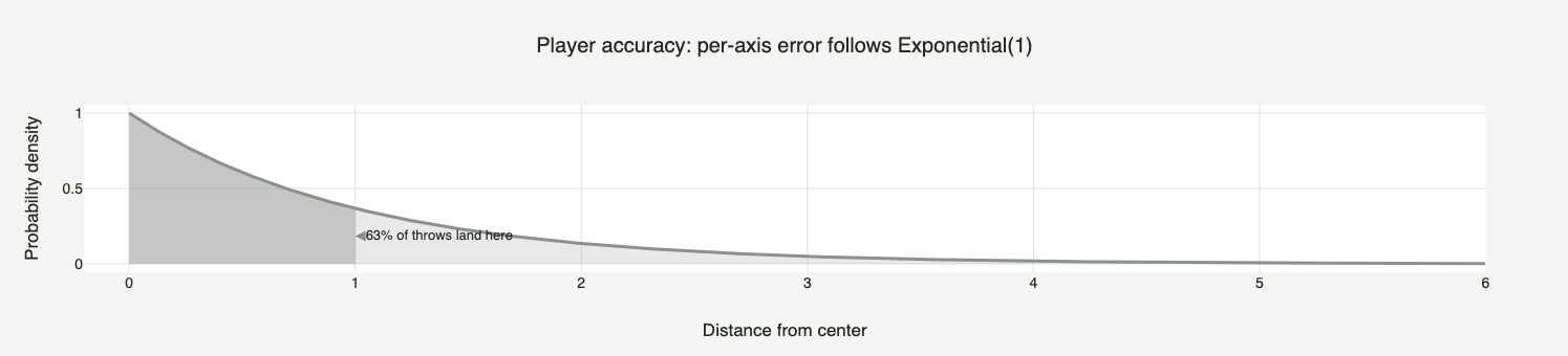
Within this framing, the mean of the original distribution is the center of the board, and the standard deviation (the scale) is the radius around which the thrower "misses" each throw. Note that this holds for any origin distribution: you can always say that the mean represents the center and the scale, the size of the error around it.

Now decompose each throw into two axes, $x$ and $y$. On each axis, the size of the error follows the origin distribution (the Exponential from Figure 1), and the direction (left or right, up or down) is decided by a coin flip. Combining magnitude and direction, the error per axis becomes a symmetric, sharply peaked curve around zero, far from a bell. The board is the $x$–$y$ plane; when you stack the frequency of the errors from both axes as height over that plane, what emerges is the bell of the Normal.

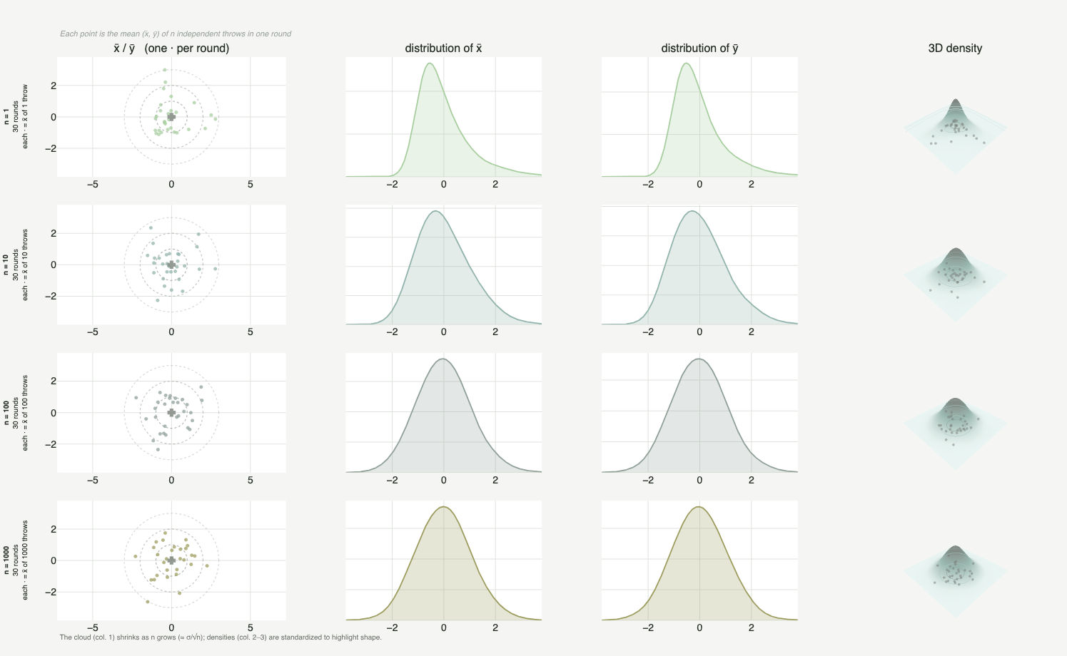
Figure 2 shows this process in action. First of all, it is worth understanding what each column represents: the 1st column (X / Y) is where the darts land on the board; the 2nd and 3rd columns (density in X and in Y) are the frequency of those errors projected onto each axis; and the 4th column (3D) is the surface that appears when you stack those two projections as height over the plane, exactly the "stack as height" described above.

The detail that ties it all together is in the rows. Each point is not a lone throw: it is the average position of the thrower over $k$ rounds (from "1 round" to "1000 rounds"). This is where the metaphor meets the $n \to \infty$ of the formal version: increasing the number of rounds is increasing the $n$ of the sample mean. Notice what happens going down the rows: the per axis density, which starts sharp and skewed (a legacy of the Exponential), keeps giving way and rounding off until it becomes the symmetric bell of the Normal. The origin is the opposite of a bell, but the mean, as we accumulate rounds, has nowhere to run.

---

The mean survives; the standard deviation transforms

I hope that bit of persuasion was enough (or at least plausible). From it we take that the mean of the original distribution is "preserved" in the new Normal. The standard deviation, on the other hand, does not carry over so directly: the standard deviation of the resulting Normal is $\sigma/\sqrt{n}$, not the original $\sigma$. That is exactly what we saw the cloud of darts do in Figure 2, shrinking with each row as the rounds increased.

The intuition is actually simple. When you sum the mean of $n$ variables, the final mean is the sum of the means divided by $n$. With the variance (and the standard deviation) the game is different: the sum of those values grows with $n$, and dividing by $\sqrt{n}$ is the way to regularize that metric in the face of the $n$ variables. It is not exactly this, but it is the intuition that holds the argument up.

And where does this $\pi$ come from?

Even after all this, one nagging question remains: "I have seen countless normal curves in my life, where does this $\pi$ come from? What does the Normal have to do with a circle?"

It really does not seem natural that a distribution which shows up all the time in nature would carry a circle baked into its definition. And why, of all distributions, is it precisely the Normal (the Gaussian, to its friends) that repeats this much? Setting aside conspiracy theories and numerology, the Gaussian has a few intriguing properties that help justify the fame.

The famous Herschel–Maxwell argument gives the intuition. Suppose you are looking for a distribution with radial symmetry in a plane ($x$ and $y$) that can be decomposed into two factors, one for each axis. The only solution that emerges is the Gaussian (here comes our first article of faith: to avoid heavy algebra, you will have to believe this statement is true). It is the same radial symmetry you saw appear in the 4th column of Figure 2: the bell that rises over the $x$–$y$ plane looks the same from any direction.

Because of that radial symmetry, a circular area appears: if you decompose the total value $r$ radially into $x$ and $y$, you land on the formula for the radius of a circle, $r^2 = x^2 + y^2$. It is from this relation that the $\pi$ appears (this is also where the famous trick of the $e^{-x^2}$ integral via polar coordinates comes in, popularly associated with Poisson). And since the 2D manipulations that solve the distribution use this radial symmetry, when you project the solution back to 1D the $\pi$ stays, only now under a square root, which is exactly the $\sqrt{2\pi}$ that lives in the denominator of the PDF.

---

Gaussian + Gaussian = Gaussian

A consequence of this same idea (interesting at least for those who made it this far; the ones who abandoned the text probably will not find it as fun): the sum of two independent Gaussian random variables is a new Gaussian variable.

It seems obvious, but there is a subtlety. Summing two variables from the same distribution generally does not preserve the distribution, although several families also have this property (Poisson, Gamma with the same scale, and even the Cauchy are closed under sums). What makes the Gaussian special is something else: it is the only stable distribution with finite variance, and it is the same radial decomposition factor that guarantees this.

From there you can risk a generalization. If you sum "infinitely many" variables (with finite variance) and believe the result should be some stable distribution, the only candidate able to stay intact throughout the process is the Gaussian (again, an article of faith). And here we meet the CLT again by another route: starting from any distribution with finite variance, by summing infinitely many variables from the same distribution you approach some limiting distribution, and the only one that does not degrade in this process is the Normal. You "deform" the distribution until it reaches the Normal and, from then on, it stays intact. (Without finite variance the destination changes: sums of heavy tailed variables, like the Cauchy, converge to other stable laws, this is the generalized CLT.)

How far can we loosen the hypotheses

The last curiosity is precisely knowing how far we can relax the initial hypotheses. You can give up independence (martingales) and even extend the theorem to high dimension: Klartag's central limit theorem for convex bodies shows that the projections (marginals) of log concave distributions in high dimension, such as the uniform distribution over a convex body, are approximately Gaussian. They are not all the roads, but many of them lead to the Normal.

If you want to learn more about this powerful theorem and how far we have already come in this branch of mathematics, it is worth going through the references below. There are proofs, resources with these and other intuitions, and a good starting point to understand, at a university level, this "magic" of statistics.

← Back to all posts

References

- Sanderson, G. (3Blue1Brown) (2023). But what is the Central Limit Theorem? [video]. YouTube.
- Sanderson, G. (3Blue1Brown) (2023). Why π is in the normal distribution (beyond integral tricks) [video]. YouTube.
- Sanderson, G. (3Blue1Brown) (2023). Convolutions | Why X+Y in probability is a beautiful mess [video]. YouTube.
- Sanderson, G. (3Blue1Brown) (2023). A pretty reason why Gaussian + Gaussian = Gaussian [video]. YouTube.
- Lindeberg, J. W. (1922). Eine neue Herleitung des Exponentialgesetzes in der Wahrscheinlichkeitsrechnung. Mathematische Zeitschrift, 15(1), 211–225.
- Feller, W. (1935). Über den zentralen Grenzwertsatz der Wahrscheinlichkeitsrechnung. Mathematische Zeitschrift, 40(1), 521–559.
- Esseen, C.-G. (1942). On the Liapunov limit of error in the theory of probability. Arkiv för Matematik, Astronomi och Fysik, A28, 1–19.
- Shevtsova, I. (2011). On the absolute constants in the Berry-Esseen type inequalities for identically distributed summands. arXiv preprint.
- Stein, C. (1972). A bound for the error in the normal approximation to the distribution of a sum of dependent random variables. Proceedings of the Sixth Berkeley Symposium on Mathematical Statistics and Probability, 2, 583–602.
- Chen, L. H. Y., Goldstein, L., & Shao, Q. M. (2011). Normal Approximation by Stein's Method. Springer.
- Billingsley, P. (1995). Probability and Measure (3rd ed.). Wiley.
- Bradley, R. C. (2007). Introduction to Strong Mixing Conditions. Kendrick Press.
- Klartag, B. (2007). A central limit theorem for convex sets. Inventiones Mathematicae, 168(1), 91–131.
- Fischer, H. (2011). A History of the Central Limit Theorem: From Classical to Modern Probability Theory. Springer.
- Le Cam, L. (1986). The Central Limit Theorem around 1935. Statistical Science, 1(1), 78–91.
- Durrett, R. (2019). Probability: Theory and Examples (5th ed.). Cambridge University Press.
- van der Vaart, A. W. (1998). Asymptotic Statistics. Cambridge University Press.
- Tao, T. (2010). 254A, Notes 2: The central limit theorem. What's New (blog).
- Tao, T. (2015). 275A, Notes 4: The central limit theorem. What's New (blog).
- Tao, T. (2015). 275A, Notes 5: Variants of the central limit theorem. What's New (blog).
- Chin, C. W. (2021). A Short and Elementary Proof of the Central Limit Theorem by Individual Swapping. arXiv preprint, arXiv:2106.00871.
- Wikipedia contributors. Central limit theorem. Wikipedia, The Free Encyclopedia.